#/local/bin/bash
#		GMT EXAMPLE 03
#
#		@(#)job03.bash	1.9  03/11/99
#
# Purpose:	Resample track data, do spectral analysis, and plot
# GMT progs:	filter1d, fitcircle, gmtset, minmax, project, sample1d,
# 		spectrum1d, trend1d, pshistogram, psxy, pstext
# Unix progs:	$AWK, cat, echo, head, paste, rm, tail
#
# This example begins with data files "ship.xyg" and "sat.xyg" which
# are measurements of a quantity "g" (a "gravity anomaly" which is an
# anomalous increase or decrease in the magnitude of the acceleration
# of gravity at sea level).  g is measured at a sequence of points "x,y"
# which in this case are "longitude,latitude".  The "sat.xyg" data were
# obtained by a satellite and the sequence of points lies almost along
# a great circle.  The "ship.xyg" data were obtained by a ship which
# tried to follow the satellite's path but deviated from it in places.
# Thus the two data sets are not measured at the same of points,
# and we use various GMT tools to facilitate their comparison.
# The main illustration (example_03.ps) are accompanied with 5 support
# plots (03a-f) showing data distributions and various intermediate steps.
#
# First, we use "fitcircle" to find the parameters of a great circle
# most closely fitting the x,y points in "sat.xyg":
#
fitcircle sat.xyg -L2 > report
cposx=`grep "L2 Average Position" report | cut -f1`
cposy=`grep "L2 Average Position" report | cut -f2`
pposx=`grep "L2 N Hemisphere" report | cut -f1`
pposy=`grep "L2 N Hemisphere" report | cut -f2`
#
# Now we use "project" to project the data in both sat.xyg and ship.xyg
# into data.pg, where g is the same and p is the oblique longitude around
# the great circle.  We use -Q to get the p distance in kilometers, and -S
# to sort the output into increasing p values.
#
project  sat.xyg -C$cposx/$cposy -T$pposx/$pposy -S -Fpz -Q > sat.pg
project ship.xyg -C$cposx/$cposy -T$pposx/$pposy -S -Fpz -Q > ship.pg
#
# The minmax utility will report the minimum and maximum values for all columns.
# We use this information first with a large -I value to find the appropriate -R
# to use to plot the .pg data.
#
cat sat.pg ship.pg | minmax -I100/25 -C > $$
xmin=`$AWK '{print $1}' $$`
xmax=`$AWK '{print $2}' $$`
ymin=`$AWK '{print $3}' $$`
ymax=`$AWK '{print $4}' $$`
gmtset MEASURE_UNIT INCH
psxy -R$xmin/$xmax/$ymin/$ymax -JX8i/5i -Ba500f100:"Distance along great circle":/a100f25:"Gravity anomaly (mGal)":WeSn -U/-1.75i/-1.25i/"Example 3a in Cookbook" -X2i -Y1.5i -K -W1p sat.pg > example_03a.ps
psxy -R -JX -O -Sp0.03i ship.pg >> example_03a.ps
#
# From this plot we see that the ship data have some "spikes" and also greatly
# differ from the satellite data at a point about p ~= +250 km, where both of
# them show a very large anomaly.
#
# To facilitate comparison of the two with a cross-spectral analysis using "spectrum1d",
# we resample both data sets at intervals of 1 km.  First we find out how the data are
# typically spaced using $AWK to get the delta-p between points and view it with
# "pshistogram".
#
$AWK '{ if (NR > 1) print $1 - last1; last1=$1; }' ship.pg | pshistogram  -W0.1 -G0 -JX3i -K -X2i -Y1.5i -B:."Ship": -U/-1.75i/-1.25i/"Example 3b in Cookbook" > example_03b.ps
$AWK '{ if (NR > 1) print $1 - last1; last1=$1; }' sat.pg  | pshistogram  -W0.1 -G0 -JX3i -O -X5i -B:."Sat": >> example_03b.ps
#
# This experience shows that the satellite values are spaced fairly evenly, with
# delta-p between 3.222 and 3.418.  The ship values are spaced quite unevelnly, with
# delta-p between 0.095 and 9.017.  This means that when we want 1 km even sampling,
# we can use "sample1d" to interpolate the sat data, but the same procedure applied
# to the ship data could alias information at shorter wavelengths.  So we have to use
# "filter1d" to resample the ship data.  Also, since we observed spikes in the ship
# data, we use a median filter to clean up the ship values.  We will want to use "paste"
# to put the two sampled data sets together, so they must start and end at the same
# point, without NaNs.  So we want to get a starting and ending point which works for
# both of them.  Thus we need to start at max( min(ship.p), min(sat.p) ) and end
# conversely.  "minmax" can't do this easily since it will return min( min(), min() ),
# so we do a little head, paste $AWK to get what we want.
#
head -1 ship.pg > ship.pg.extr
head -1 sat.pg > sat.pg.extr
paste ship.pg.extr sat.pg.extr | $AWK '{ if ($1 > $3) print int($1); else print int($3); }' > sampr1
tail -1 ship.pg > ship.pg.extr
tail -1 sat.pg > sat.pg.extr
paste ship.pg.extr sat.pg.extr | $AWK '{ if ($1 < $3) print int($1); else print int($3); }' > sampr2
sampr1=`cat sampr1`
sampr2=`cat sampr2`
#
# Now we can use sampr in $AWK to make a sampling points file for sample1d:
$AWK 'BEGIN { for (i='$sampr1'; i <= '$sampr2'; i++) print i }' /dev/null > samp.x
#
# Now we can resample the projected satellite data:
#
sample1d sat.pg -Nsamp.x > samp_sat.pg
#
# For reasons above, we use filter1d to pre-treat the ship data.  We also need to sample it
# because of the gaps > 1 km we found.  So we use filter1d | sample1d.  We also use the -E
# on filter1d to use the data all the way out to sampr1/sampr2 :
#
filter1d ship.pg -Fm1 -T$sampr1/$sampr2/1 -E | sample1d -Nsamp.x > samp_ship.pg
#
# Now we plot them again to see if we have done the right thing:
#
psxy -R$xmin/$xmax/$ymin/$ymax -JX8i/5i -Ba500f100:"Distance along great circle":/a100f25:"Gravity anomaly (mGal)":WeSn -X2i -Y1.5i -K -W1p samp_sat.pg -U/-1.75i/-1.25i/"Example 3c in Cookbook" > example_03c.ps
psxy -R -JX -O -Sp0.03i samp_ship.pg >> example_03c.ps
#
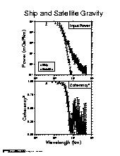
# Now to do the cross-spectra, assuming that the ship is the input and the sat is the output
# data, we do this:
#
paste samp_ship.pg samp_sat.pg | cut -f2,4 | spectrum1d -S256 -D1 -W -C >& /dev/null
#
# Now we want to plot the spectra.  The following commands will plot the ship and sat
# power in one diagram and the coherency on another diagram,  both on the same page.
# Note the extended use of pstext and psxy to put labels and legends directly on the plots.
# For that purpose we often use -Jx1i and specify positions in inches directly:
#
psxy spectrum.coh -Ba1f3p:"Wavelength (km)":/a0.25f0.05:"Coherency@+2@+":WeSn -JX-4il/3.75i -R1/1000/0/1 -U/-2.25i/-1.25i/"Example 3d in Cookbook" -P -K -X2.5i -Sc0.07i -G0 -Ey/2 -Y1.5i > example_03.ps
echo "3.85 3.6 18 0.0 1 11 Coherency@+2@+" | pstext -R0/4/0/3.75 -Jx1i -O -K >> example_03.ps
cat << END > box.d
2.375	3.75
2.375	3.25
4	3.25
END
psxy -R -Jx -O -K -W1.5p box.d >> example_03.ps
psxy -St0.07i -O -Ba1f3p/a1f3p:"Power (mGal@+2@+km)"::."Ship and Satellite Gravity":WeSn spectrum.xpower -R1/1000/0.1/10000 -JX-4il/3.75il -Y4.2i -K -Ey/2 >> example_03.ps
psxy spectrum.ypower -R -JX -O -K -G0 -Sc0.07i -Ey/2 >> example_03.ps
echo "3.9 3.6 18 0.0 1 11 Input Power" | pstext -R0/4/0/3.75 -Jx -O -K >> example_03.ps
psxy -R -Jx -O -K -W1.5p box.d >> example_03.ps
psxy -R -Jx -O -K -G240 -L -W1.5p << END >> example_03.ps
0.25	0.25
1.4	0.25
1.4	0.9
0.25	0.9
END
echo "0.4 0.7" | psxy -R -Jx -O -K -St0.07i -G0 >> example_03.ps
echo "0.5 0.7 14 0.0 1 5 Ship" | pstext -R -Jx -O -K >> example_03.ps
echo "0.4 0.4" | psxy -R -Jx -O -K -Sc0.07i -G0 >> example_03.ps
echo "0.5 0.4 14 0.0 1 5 Satellite" | pstext -R -Jx -O >> example_03.ps
#
# Now we wonder if removing that large feature at 250 km would make any difference.
# We could throw away a section of data with $AWK or sed or head and tail, but we
# demonstrate the use of "trend1d" to identify outliers instead.  We will fit a
# straight line to the samp_ship.pg data by an iteratively-reweighted method and
# save the weights on output.  Then we will plot the weights and see how things
# look:
#
trend1d -Fxw -N2r samp_ship.pg > samp_ship.xw
psxy -R$xmin/$xmax/$ymin/$ymax -JX8i/4i -Ba500f100:"Distance along great circle":/a100f25:"Gravity anomaly (mGal)":WeSn -U/-1.75i/-1.25i/"Example 3e in Cookbook" -X2i -Y1.5i -K -Sp0.03i samp_ship.pg > example_03d.ps
psxy -R$xmin/$xmax/0/1.1 -JX8i/1.1i -O -Y4.25i -Bf100/a0.5f0.1:"Weight":Wesn -Sp0.03i samp_ship.xw >> example_03d.ps
#
# From this we see that we might want to throw away values where w < 0.6.  So we try that,
# and this time we also use trend1d to return the residual from the model fit (the
# de-trended data):
trend1d -Fxrw -N2r samp_ship.pg | $AWK '{ if ($3 > 0.6) print $1, $2 }' | sample1d -Nsamp.x > samp2_ship.pg
trend1d -Fxrw -N2r samp_sat.pg  | $AWK '{ if ($3 > 0.6) print $1, $2 }' | sample1d -Nsamp.x > samp2_sat.pg
#
# We plot these to see how they look:
#
cat samp2_sat.pg samp2_ship.pg | minmax -I100/25 -C > $$
xmin=`$AWK '{print $1}' $$`
xmax=`$AWK '{print $2}' $$`
ymin=`$AWK '{print $3}' $$`
ymax=`$AWK '{print $4}' $$`
psxy -R$xmin/$xmax/$ymin/$ymax -JX8i/5i -Ba500f100:"Distance along great circle":/a50f25:"Gravity anomaly (mGal)":WeSn -U/-1.75i/-1.25i/"Example 3f in Cookbook" -X2i -Y1.5i -K -W1p samp2_sat.pg > example_03e.ps
psxy -R -JX -O -Sp0.03i samp2_ship.pg >> example_03e.ps
#
# Now we do the cross-spectral analysis again.  Comparing this plot (example_03f.ps) with
# the previous one (example_03.ps) we see that throwing out the large feature has reduced
# the power in both data sets and reduced the coherency at wavelengths between 20--60 km.
#
paste samp2_ship.pg samp2_sat.pg | cut -f2,4 | spectrum1d -S256 -D1 -W -C >& /dev/null
#
psxy spectrum.coh -Ba1f3p:"Wavelength (km)":/a0.25f0.05:"Coherency@+2@+":WeSn -JX-4il/3.75i -R1/1000/0/1 -U/-2.25i/-1.25i/"Example 3g in Cookbook" -P -K -X2.5i -Sc0.07i -G0 -Ey/2 -Y1.5i > example_03f.ps
echo "3.85 3.6 18 0.0 1 11 Coherency@+2@+" | pstext -R0/4/0/3.75 -Jx -O -K >> example_03f.ps
cat << END > box.d
2.375	3.75
2.375	3.25
4	3.25
END
psxy -R -Jx -O -K -W1.5p box.d >> example_03f.ps
psxy -St0.07i -O -Ba1f3p/a1f3p:"Power (mGal@+2@+km)"::."Ship and Satellite Gravity":WeSn spectrum.xpower -R1/1000/0.1/10000 -JX-4il/3.75il -Y4.2i -K -Ey/2 >> example_03f.ps
psxy spectrum.ypower -R -JX -O -K -G0 -Sc0.07i -Ey/2 >> example_03f.ps
echo "3.9 3.6 18 0.0 1 11 Input Power" | pstext -R0/4/0/3.75 -Jx -O -K >> example_03f.ps
psxy -R -Jx -O -K -W1.5p box.d >> example_03f.ps
psxy -R -Jx -O -K -G240 -L -W1.5p << END >> example_03f.ps
0.25	0.25
1.4	0.25
1.4	0.9
0.25	0.9
END
echo "0.4 0.7" | psxy -R -Jx -O -K -St0.07i -G0 >> example_03f.ps
echo "0.5 0.7 14 0.0 1 5 Ship" | pstext -R -Jx -O -K >> example_03f.ps
echo "0.4 0.4" | psxy -R -Jx -O -K -Sc0.07i -G0 >> example_03f.ps
echo "0.5 0.4 14 0.0 1 5 Satellite" | pstext -R -Jx -O >> example_03f.ps
#
\rm -f $$ box.d report samp* *.pg *.extr spectrum.* .gmtcommands
